#MAixPy: Object detector - MobileNet and YOLOv2 on Sipeed MAix Dock

This tutorial is about training (on PC) and deploying a YOLOv2 object detector on a MAix M1w Dock Suit running MicroPython. The MobileNet is used as a pre-trained model for the training.

Therefore, this tutorial will try to accomplish the following points:

1. A quick introduction to YOLO(v2)
2. A quick introduction to MAix KPU
3. Training, evaluation, and testing of the object detector model (on Jupyter-Notebooks running on Docker)
4. Flashing the trained model on the MAix M1w Dock Suit running MicroPython (MAixPy)
5. Detecting a BRIO locomotive using the MAix M1w Dock Suit

A training example is included, which is used in the following video (turn on the sound!).

Software and Hardware

The following hardware and software will be used in this tutorial:

YOLO

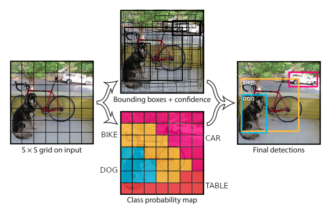
The high-level idea behind You Only Look Once (YOLO) is to apply a single neural network to the full image to detect and classify objects. Therefore, the YOLO splits the image into regions (grid) and for each region, bounding boxes, confidences and class probabilities are calculated and predicted.

To explain YOLO, I use the example of the original paper. To start, you need to define these 3 main parameters:

• S: number of grid cells (S×S) to divide an image
• B: number of bounding boxes that each grid cell will predict/calculate
• C: number of different classes that can be predicted on each grid cell

Fig. 1: The detector divides the image into an S×S grid and for each grid cell predicts B bounding boxes, confidence for those boxes, and C class probabilities. The predictions are encoded as an S×S×(B×5+C) tensor. (Image and legend taken from source and a bit modified)

As you can see in the left subfigure of Fig. 1, an image is divided into 7×7 grid cells (S=7) and each cell generates two bounding boxes (B=2) with the confidences described by the thickness of the box borders (Fig. 1 mid-upper position). The confidence defines the probability that the bounding box contains an object (check e.g. the bounding boxes surrounding the white car -top right). Thus, at this point, you know where the objects in the image are, but you don't know what they are. Therefore, each cell predicts also a class probability (Fig. 1 mid-lower position). This is a conditioned probability on an object (e.g. P(Car|Object)). This means, if a grid cell predicts a car, it is saying: if there is an object in this grid cell, then that object is a car. In the paper's example, 20 classes of objects were detected (C=20) Then, combining the box and the class predictions results in 1470 tensors/outputs (7×7×(2×5+20) = 1470 tensors). Thresholding the tensors (e.g. confidence greater than 30%) results in the final detections presented in the right subfigure of Fig. 1.

The original paper was published in May 2016, and the talk is available on Youtube. The training is also explained in the video/paper.

Same authors published YOLOv2 some months later (Dec. 2016) and YOLOv3 in April 2018. YOLOv2 and YOLOv3 are improvements of the original YOLO detector. A comparison of the detectors can be found in this video.

MAix KPU

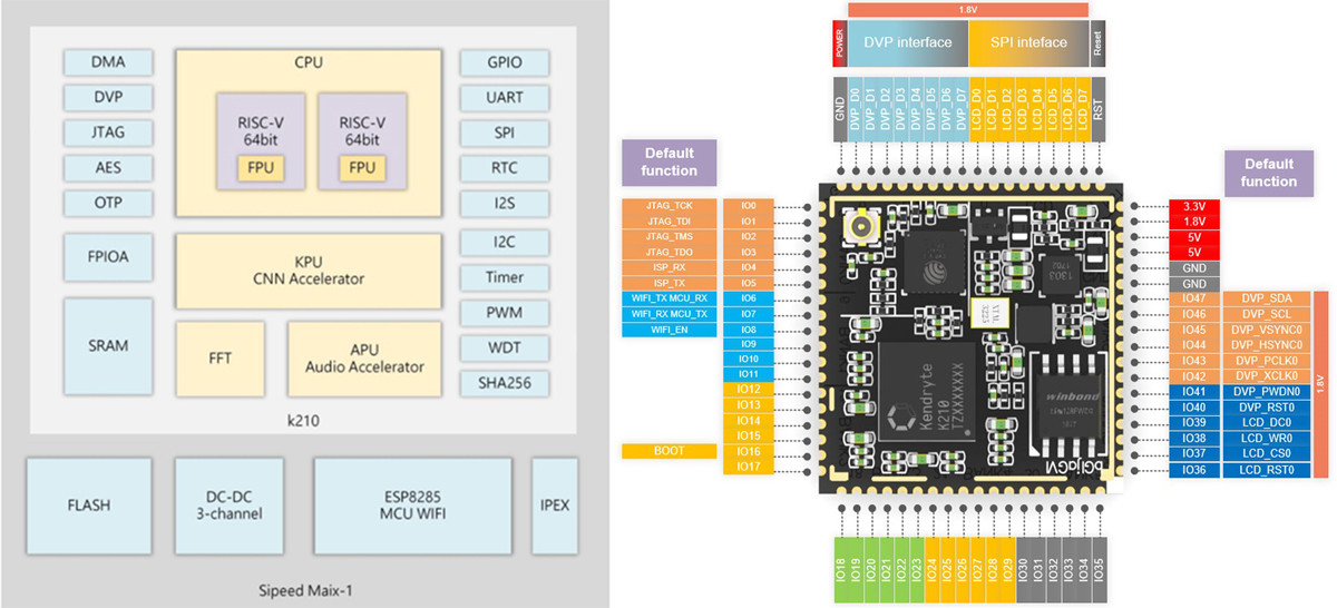
MAix is a Sipeed module designed to run AI at the edge (AIoT). It results in a lower cost and power solution than a combination of an ARM + edgeTPU like the Google Coral products (but of course with more limitations too).

Fig. 2: MAix's modules (source)

The Sipeed MAix has a KPU (see Fig 2), which is a general-purpose neural network processor that can do convolutional neural network calculation at low power consumption. The KPU can obtain the size, coordinates, and types of detected objects (object detector) or detect and classify faces and objects (object classification).

And if you look through the documentation, you can find that YOLOv2 is implemented and can be used to detect objects on images recorded with the OV2640 camera.

Therefore, the next steps in this tutorial are to train a model using Tensorflow, convert it to Tensorflow Lite and using nncase export it into a .kmodel that can be flash on the MAix Dock M1w suit and then loaded using MicroPython to detect and classify objects.

Object Detector Model

Docker and Libraries

Install Docker on your machine and create a notebooks folder inside e.g. Documents/:

curl -sSL https://get.docker.com | sh
mkdir ~/Documents/notebooks/

Then, deploy the tensorflow/tensorflow:latest-py3-jupyter image using:

sudo docker run -d -p 8888:8888 -v ~/Documents/notebooks/:/tf/notebooks/ tensorflow/tensorflow:latest-py3-jupyter

I explained the -v flag here: It is a "Bind Mount". This means the ~/Documents/notebooks/ folder is connected to the /notebooks/ folder inside the container. This makes the data inside the folder /tf/notebooks/ (container) persistent. Otherwise, if the container is stopped you lose the files.

Then, clone the repository inside ~/Documents/notebooks/

cd ~/Documents/notebooks/
git clone https://github.com/lemariva/MaixPy_YoloV2

Open the following URL in your host web browser: http://localhost:8888. You need a token to log in. The token is inside the container. To get it, list the running containers to get the container ID with the following command:

$ docker container ls
CONTAINER ID        IMAGE    [....]
5082a85283bb        tensorflow/  [....]

Then, read the logs typing:

$ docker logs 5082a85283bb

[...]
The Jupyter Notebook is running at:
[...] http://ac64d540a1cb:8888/?token=df050fa3b53de5f9203ca862e5f3656962b665dc224243a8
[...]

The hash after token= is the token needed to log in.

Model Training, Evaluation, and Test

I added a training example, in which I used the BRIO locomotive. You can train the model again using the Jupyter Notebook: training.ipynb. The (hyper)parameters for the training are loaded from configs/brio.json.

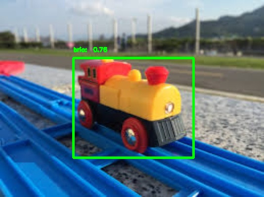
To evaluate the model, copy the weights.h5 file inside the brio/ folder and open the Jupyter Notebook: evaluation.ipynb. The Notebook loads the model, takes the images inside datasets/brio/images_test/, evaluates them and saves the results under evaluation/detected/. An example of those images looks like Fig. 3.

Fig. 3: BRIO 33594 detected with 0.76 of confidence!

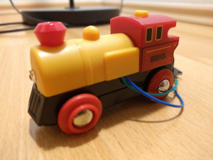
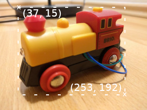
To train a new model, you need to create a json file inside e.g. the configs/ folder. You can use configs/brio.json as a reference. Additionally, you need to have enough images (e.g. datasets/brio/images/brio_8.jpg) and you need to create an annotation file (datasets/brio/xml/brio_8.xml) for each image. The annotation file for the image brio_8.jpg (Fig. 4a) looks like this:

<annotation verified="yes">
    <folder>images</folder>
    <filename>brio_8.jpg</filename>
    <path>/notebooks/MaixPy_YoloV2/data/brio/images/brio_8.jpg</path>
    <source>
        <database>Unknown</database>
    </source>
    <size>
        <width>300</width>
        <height>225</height>
        <depth>3</depth>
    </size>
    <segmented>0</segmented>
    <object>
        <name>brio</name>
        <pose>Unspecified</pose>
        <truncated>0</truncated>
        <difficult>0</difficult>
        <bndbox>
            <xmin>37</xmin>
            <ymin>15</ymin>
            <xmax>253</xmax>
            <ymax>192</ymax>
        </bndbox>
    </object>
</annotation>

Change the folder, filename and path first. After that, set the image size and the coordinates of the boundary box (bndbox) in which the object is located (see Fig. 4b). You can also define the pose, truncated and difficult parameters to get a better detection. This final step is optional, but it can help a lot.

Fig. 4a: brio_8.jpg from the training set	Fig. 4b: Image & boundary box (brio_8.xml)

After labelling the images, divide them into two sets: training (e.g. brio/images/, brio/xml/) and evaluation (e.g. brio/images_valid/, brio/xml_valid/ ) and take a couple of other images for a test set (you don't need annotation files for these ones). The paths for the sets are defined in the config file (configs/brio.xml).

You can also play with the hyperparameters in the config file such as the actual_epoch, batch_size, learning_rate, anchors or train_times. They will influence the final performance of the model. For example, if you have a larger dataset containing more training images and more detection classes, you should train your model by more epochs (actual_epoch) for better convergence. Or, if the targeting objects inside your image are typically small, you can use smaller anchors' parameters (anchors). This defines the prior anchors for the detector (YOLOv2). If you don't have a lot of images, you can use a higher train_times to improve the training or set jitter to true. This enables image augmentation: resizing, shifting and blurring of the images to prevent overfitting and to have more variety in the dataset. It also flips the image randomly. However, set it to false, if your objects are orientation-sensitive.

More info about the hyperparameters can be found in the YOLOv2 paper.

Save Model as tflite

After training the model, you get two files: weights.h5 and weights.tflite. The second file is a conversion of the Tensorflow model to Tensorflow lite, and this can be converted to a kmodel that can be loaded on the Sipeed MAix board.

I've updated the original repository to Tensorflow 2.0. The file yolo/backend/utils/fit.py save the tflite model (def save_tflite(model):). Tensorflow 2.0 has a direct function to convert a Tensorflow model to a tflite model.

converter = tf.lite.TFLiteConverter.from_keras_model(model)
tflite_model = converter.convert()
file = open ("weights.tflite" , "wb")
file.write(tflite_model)

However, the resulting file can only be converted to a kmodel using a version of nncase greater than 0.2.0. Otherwise, you get the following error:

Fatal: Layer TensorflowReshape is not supported
[...]

If you use nncase v.0.2.0 you get a V4 kmodel, which is nowadays not compatible with the KPU library (only V3) that runs on MicroPython. Trying to load a V4 model on the KPU gives you the following error:

v=1263354956, flag=4, arch=0, layer len=1, mem=1926400, out cnt=127
err: we only support V3 now, get V1263354956

Thus, you need to use nncase v0.1.0 RC5 and you have to convert the Tensorflow model using following code:

model.save("weights.h5", include_optimizer=False)
tf.compat.v1.disable_eager_execution()
converter = tf.compat.v1.lite.TFLiteConverter.from_keras_model_file("weights.h5",
                                    output_arrays=['detection_layer_30/BiasAdd'])
tflite_model = converter.convert()
file = open ("weights.tflite" , "wb")
file.write(tflite_model)

Both options are included in the yolo/backend/utils/fit.py file. The second option is only active.

Convert tflite to kmodel model

First of all, get the MAix toolbox from the GitHub repo:

git clone https://github.com/sipeed/Maix_Toolbox.git

and fix a small bug inside the file get_nncase.sh

cd Maix_Toolbox
nano get_nncase.sh
​
//inside the get_nncase.sh
...
...
tar -Jxf ncc-linux-x86_64.tar.xz
rm ncc-linux-x86_64.tar.xz
...
//end of file

Then, download the library nncase typing:

./get_nncase.sh

To convert the model, nncase needs some example images for inference. These example images have to be the same resolution as the input image's resolution to your model. The input size is defined in the configuration file brio.json as:

{
    "model" : {
        "architecture":         "MobileNet",
        "input_size":           224,
        [...]
        }
}

I included some examples inside the folder datasets/brio/images_maixpy. The images' sizes are 224x224 pixels. Put these images in a images folder inside Maix_Toolbox and copy also the weights.tflite file to the Maix_Toolbox folder. Finally, convert the Tensorflow Lite model to a .kmodel using:

./tflite2kmodel.sh weights.tflite

If you successfully convert the model, you will get a weights.kmodel file and you will see:

usage: ./tflite2kmodel.sh xxx.tflite
2020-01-12 13:53:03.608486: I tensorflow/core/platform/cpu_feature_guard.cc:141] Your CPU supports instructions that this TensorFlow binary was not compiled to use: SSE4.1 SSE4.2 AVX AVX2 FMA
0: InputLayer -> 1x3x224x224
1: K210Conv2d 1x3x224x224 -> 1x24x112x112
[...]
30: OutputLayer 1x30x7x7
KPU memory usage: 2097152 B
Main memory usage: 7352 B

This shows you some details of the YOLOv2 model: I/O dimension of InputLayer, OutputLayer, and each Conv2d layer, as well as the memory usage of the converted model.

Get the MAix board ready

First, you need to flash MicroPython on the Sipeed M1w Dock suit. Then, you can upload the model and load it as a file, or you can flash it and load it from its memory position.

Flash MicroPython (MAixPY)

You can download a pre-compiled firmware (MAixPY) or you can compile the MAixPY from scratch. To compile the firmware from scratch (on Ubuntu), clone the following repository:

git clone https://github.com/sipeed/MaixPy
cd MaixPy
git submodule update --recursive --init

Install the requirements:

sudo apt update
sudo apt install python3 python3-pip build-essential cmake
sudo pip3 install -r requirements.txt

Download and install the kendryte toolchain:

wget http://dl.cdn.sipeed.com/kendryte-toolchain-ubuntu-amd64-8.2.0-20190409.tar.xz
sudo tar -Jxvf kendryte-toolchain-ubuntu-amd64-8.2.0-20190409.tar.xz -C /opt

The toolchain should be under /opt, otherwise you need to change the path inside config_defaults.mk.

Then, connect the Sipeed M1w Dock suit to a USB port on your host machine and type the following:

cd MaixPy/projects/maixpy_k210_minimum
python3 project.py menuconfig
python3 project.py build
python3 project.py flash -B dan -b 1500000 -p /dev/ttyUSB0 -t

If you want to flash a pre-compiled firmware, follow the steps described here, or use the kflash tool.

Flash the kmodel

As I mentioned, it is possible to upload the kmodel and upload it to the KPU, or you can flash a kfpkg file and point the KPU to the memory address where you flashed it. I got some problems uploading the model as a file (1.9 MB), thus, I recommend to flash it.

First, clone the kflash.py tool using:

git clone https://github.com/sipeed/kflash.py.git

kflash.py doesn't have the option to flash a file with an address offset, so you'll need to make a .kfpkg file. A .kfpkg package is just a .zip file with a custom extension that contains the following files:

• flash-list.json: json file describing the files included in the package
• *.kmodel: – the model that will be flashed

The file flash-list.json looks like this:

{
  "version": "0.1.0",
  "files": [
    {
      "address": 0x00300000,
      "bin": "m.kmodel",
      "sha256Prefix": false
    }
  ]
}

You can find an example of the .kfpkg file inside the repo: lemariva/uPyMaixYoloV2.

Download the example and replace the m.kmodel inside with your weights.kmodel file (rename it before). Then, flash the model.kfpkg file to the MAix using:

./kflash.py -p /dev/ttyUSB0 -b 2000000 model.kfpkg

Run the object detector

The repository lemariva/uPyMaixYoloV2 includes an example to run the object detector on the Sipeed M1w Dock suit (includes Wi-Fi).

Clone the repository:

git clone https://github.com/lemariva/uPyMaixYoloV2

and Open the Folder using VSCode. You can connect to the board using the PyMakr extension. I wrote a tutorial for the ESP/WiPy boards but the extension can be also used with the MAix. However, you can only run files but you cannot upload them.

Before you run the file, configure your Wi-Fi credentials:

# wlan access
ssid_ = ""
wpa2_pass = ""

or remove the lines between # wlan access and ## Sensor, if you don't want to connect the board to Wi-Fi.

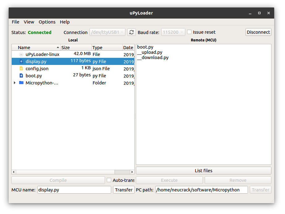
If you want to upload the boot.py file to the board, you can use uPyLoader. First, clone the repository:

git clone https://github.com/BetaRavener/uPyLoader.git

and install the following dependencies:

pip3 install PyQt5

Then:

1. Start the application: python main.py you'll see something like Fig. 5
2. Select the serial port and click on the Connect button to connect the board.
3. The first time you run the software, you need to initialize it:
   • Go to File->Init transfer files to complete the initialization. This creates two files on the board, __upload.py and __download.py.
4. Select the file that you want to upload (e.g. boot.py), and click on the Transfer button.

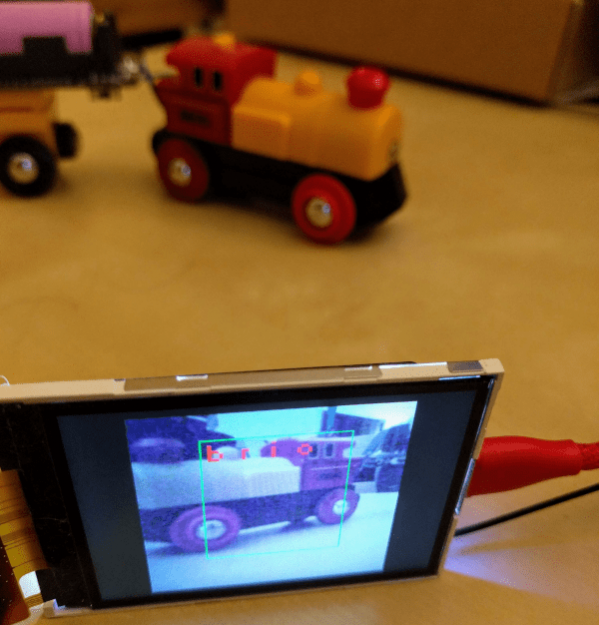
Fig. 5: uPyLoader connected to the MaixPy

Then, you can disconnect the board from the USB port, the next time that you start it, the object detector will run and you'll get something like Fig. 6.

Fig. 6: Object detector working: BRIO locomotive detected!

Conclusions

This tutorial explains how to train, evaluate, test and deploy an object detector on a MAix Dock M1w. The object detector is a YOLOv2 and uses MobileNet as base architecture. An example for you is included, in which the MobileNet is extended to detect a BRIO locomotive. The model is trained using Tensorflow 2.0 with Keras, it is then converted to Tensorflow Lite and finally to a KModel that can be loaded on the KPU unit of the Sipeed M1w Dock suit to detect the trained object. The training, evaluation and test codes are implemented on Jupyter Notebooks and can be run inside a tensorflow/tensorflow:latest-py3-jupyter container.